理解 RNN

循环神经网络 (Recurrent Neural Network, RNN) 是一种用于处理时间序列数据的神经网络结构。包括文字、语音、视频等对象。这些数据有两个主要特点：

数据无固定长度
数据是有时序的，相邻数据之间存在相关性，非相互独立

考虑这样一个问题，如果要预测句子下一个单词是什么，一般需要用到当前单词以及前面的单词，因为句子中前后单词并不是独立的。比如，当前单词是“很”，前一个单词是“天空”，那么下一个单词很大概率是“蓝”。循环神经网络就像人一样拥有记忆的能力，它的输出依赖于当前的输入和记忆，刻画出一个序列当前的输出与之前信息的关系。

循环神经网络适用于许多序列问题中，例如文本处理、语音识别以及机器翻译等。

基本结构

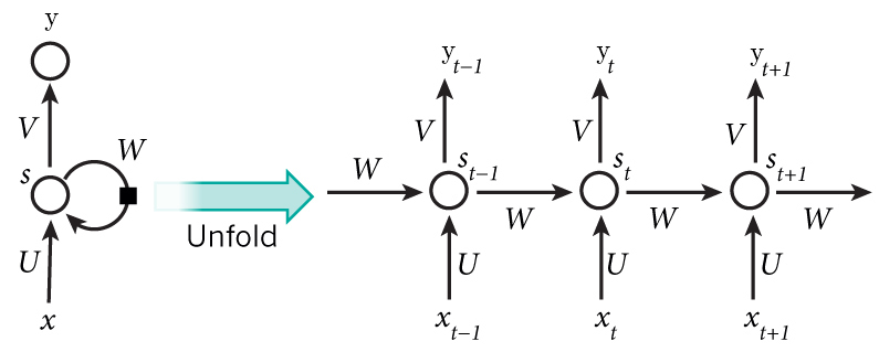
如果把上面有 W 的那个带箭头的圈去掉，它就变成了普通的全连接神经网络。图中每个圆圈可以看作是一个单元，而且每个单元做的事情也是一样的，因此可以折叠呈左半图的样子。用一句话解释 RNN，就是一个单元结构重复使用。

简单理清一下各符号的定义：

$x_t$ 表示 t 时刻的输入
$y_t$ 表示 t 时刻的输出
$s_t$ 表示 t 时刻的记忆，即隐藏层的输出
U 是输入层到隐藏层之间的权重矩阵
W 是记忆单元到隐藏层之间的权重矩阵
V 是隐藏层到输出层之间的权重矩阵
U, W, V 都是权重矩阵，在不同时刻 t 之间是共享权重的

从右半图可以看到，RNN 每个时刻隐藏层输出都会传递给下一时刻，因此每个时刻的网络都会保留一定的来自之前时刻的历史信息，并结合当前时刻的网络状态一并再传给下一时刻。

比如在文本预测中，文本序列为 “machine”，则输入序列和标签序列分别为 “machin” 和 “achine”，网络的概览图如下：

前向计算

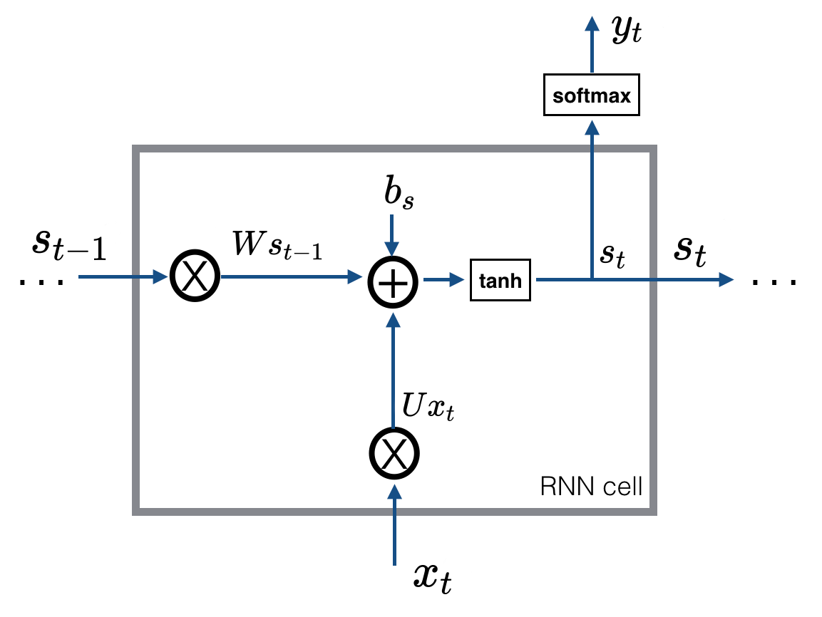
在一个循环神经网络中，假设隐藏层只有一层。在 t 时刻神经网络接收到一个输入 $x_t$，则隐藏层的输出 $s_t$ 为： $$ s_t = \tanh(Ux_t + Ws_{t-1} + b_s) $$

在神经网络刚开始训练时，记忆单元中没有上一时刻的网络状态，这时候 $s_{t-1}$ 就是一个初始值。

在得到隐藏层的输出后，神经网络的输出 $y_t$ 为： $$ y_t = \mathrm{softmax}(Vs_t + b_y) $$

设 t 时刻的输入 $x_t$ 的维度为 $(n_x, m)$，其中 $n_x$ 为变量 $x$ 的维度（输入层节点数量），$m$ 为样本数量；隐藏层节点的数量为 $n_s$；输出层节点数量为 $n_y$。则各变量的信息如下：

变量	说明	维度
$x_t$	t 时刻输入	$(n_x, m)$
$s_t$	t 时刻隐藏层输出	$(n_s, m)$
$U$	输入层到隐藏层之间的权重矩阵	$(n_s, n_x)$
$W$	记忆单元到隐藏层之间的权重矩阵	$(n_s, n_s)$
$V$	隐藏层到输出层之间的权重矩阵	$(n_y, n_s)$
$b_s$	隐藏层偏置量	$(n_s, 1)$
$b_y$	输出层偏置量	$(n_y, 1)$

某个时刻的 RNN 前向计算流程如下：

def rnn_cell_forward(xt, s_prev, parameters):
    """
    Implements a single forward step of the RNN-cell

    Arguments:
    xt -- Your input data at timestep "t", numpy array of shape (n_x, m).
    s_prev -- Hidden state at timestep "t-1", numpy array of shape (n_s, m)
    parameters -- Python dictionary containing:
        U -- Weight matrix multiplying the input, numpy array of shape (n_s, n_x)
        W -- Weight matrix multiplying the hidden state, numpy array of shape (n_s, n_s)
        V -- Weight matrix relating the hidden-state to the output, numpy array of shape (n_y, n_s)
        bs -- Bias, numpy array of shape (n_s, 1)
        by -- Bias relating the hidden-state to the output, numpy array of shape (n_y, 1)
    
    Returns:
    s_next -- Next hidden state, of shape (n_s, m)
    yt_pred -- Prediction at timestep "t", numpy array of shape (n_y, m)
    cache -- Tuple of values needed for the backward pass, contains (s_next, s_prev, xt, parameters)
    """
    U = parameters["U"]
    W = parameters["W"]
    V = parameters["V"]
    bs = parameters["bs"]
    by = parameters["by"]

    # Compute next hidden state
    s_next = np.tanh(np.dot(W, s_prev) + np.dot(U, xt) + bs)
    # Compute output of the current cell
    yt_pred = softmax(np.dot(V, s_next) + by)
    # Store values needed for backward propagation in cache
    cache = (s_next, s_prev, xt, parameters)
    return s_next, yt_pred, cache

接下来考虑沿时间线前向计算的过程，设总的时间步长为 $T_x$，此时网络的输入 $x$ 的维度为 $(n_x, m, T_x)$，$s_0$ 为初始隐藏状态，可以使用一些策略进行初始化：

置 0
随机值
作为模型参数训练学习

通常采用零向量或随机向量作为初始状态，但通过学习得出的初始值可能效果更好，见 6。

def rnn_forward(x, s0, parameters):
    """
    Implement the forward propagation of the recurrent neural network

    Arguments:
    x -- Input data for every time-step, of shape (n_x, m, T_x).
    s0 -- Initial hidden state, of shape (n_s, m)
    parameters -- See `rnn_cell_forward`

    Returns:
    s -- Hidden states for every time-step, numpy array of shape (n_s, m, T_x)
    y_pred -- Predictions for every time-step, numpy array of shape (n_y, m, T_x)
    caches -- Tuple of values needed for the backward pass, contains (list of caches, x)
    """
    
    # Initialize "caches" which will contain the list of all caches
    caches = []
    
    n_x, m, T_x = x.shape
    n_y, n_s = parameters["V"].shape

    s = np.zeros((n_s, m, T_x))
    y_pred = np.zeros((n_y, m, T_x))
    
    s_next = s0
    # loop over all time-steps
    for t in range(T_x):
        # Update next hidden state, compute the prediction
        s_next, yt_pred, cache = rnn_cell_forward(x[:,:,t], s_next, parameters)
        s[:,:,t] = s_next
        y_pred[:,:,t] = yt_pred
        caches.append(cache)
            
    caches = (caches, x)
    return s, y_pred, caches

反向传播

关于梯度的计算，我们先计算隐藏层输出 $s_t$ 的梯度，然后根据链式法则求得其他梯度。对于某时刻的隐藏层输出 $s_t$，误差的来源有两个：一个是当前时刻的输出层传递过来的误差，另一个是后面时刻的输出层传递过来的误差。总的来说，就是把大于等于 t 时刻的所有误差都计算进去。

例如，考虑 t - 3 时刻的梯度计算：

$$ \begin{aligned} \frac{\partial E}{\partial s_{t-3}} &= \frac{\partial L}{\partial s_{t}} \frac{\partial s_t}{\partial s_{t-1}}\frac{\partial s_{t-1}}{\partial s_{t-2}} \frac{\partial s_{t-2}}{\partial s_{t-3}} + \frac{\partial L}{\partial s_{t-1}} \frac{\partial s_{t-1}}{\partial s_{t-2}} \frac{\partial s_{t-2}}{\partial s_{t-3}} + \frac{\partial L}{\partial s_{t-2}} \frac{\partial s_{t-2}}{\partial s_{t-3}} + \frac{\partial L}{\partial s_{t-3}}\\ &=\frac{\partial s_{t-2}}{\partial s_{t-3}} \left(\frac{\partial L}{\partial s_{t}} \frac{\partial s_t}{\partial s_{t-1}}\frac{\partial s_{t-1}}{\partial s_{t-2}} + \frac{\partial L}{\partial s_{t-1}} \frac{\partial s_{t-1}}{\partial s_{t-2}} + \frac{\partial L}{\partial s_{t-2}} \right) + \frac{\partial E}{\partial s_{t-3}}\\ &=\frac{\partial E}{\partial s_{t-2}}\frac{\partial s_{t-2}}{\partial s_{t-3}} + \frac{\partial L}{\partial s_{t-3}} \end{aligned} $$

可以看出这是梯度的递归式，最后梯度的两项和上面的描述一致。我们只要从最后的 t 时刻一步一步往前面的时刻推算，就能得到所有时刻的梯度。上式还有一项需要计算，由于 $$ \frac{\partial \tanh(x)}{\partial x} = 1 - \tanh(x)^2 $$

参照前向计算中 $s_t$ 的表达式，则 $s_t$ 关于上一时刻 $s_{t-1}$ 的导数容易求得： $$ \frac{\partial s_{t}}{\partial s_{t-1}} = W^T(1 - s_t^2) $$

最后可得各权重的梯度： $$ \frac{\partial s_{t}}{\partial W} = (1 - s_t^2)s_{t-1}^T $$ $$ \frac{\partial s_{t}}{\partial U} = (1 - s_t^2)x_{t}^T $$ $$ \frac{\partial s_{t}}{\partial b_s} = \sum_{batch} (1 - s_t^2) $$

具体实现方面，可以分为两部分，一部分是单个 RNN 单元里面的反向传播；另一部分是沿时间线的反向传播。

单元内传播

设当前单元的时刻为 t，我们假设此时已经计算出了当前隐藏层输出 $s_t$ 的梯度 $\frac{\partial E}{\partial s_t}$，各权重的梯度可以立刻得出： $$ \frac{\partial E}{\partial W} = \frac{\partial E}{\partial s_t} \frac{\partial s_{t}}{\partial W} = \frac{\partial E}{\partial s_t} (1 - s_t^2)s_{t-1}^T $$ $$ \frac{\partial E}{\partial U} = \frac{\partial E}{\partial s_t} \frac{\partial s_{t}}{\partial U} = \frac{\partial E}{\partial s_t} (1 - s_t^2)x_{t}^T $$ $$ \frac{\partial E}{\partial b_s} = \frac{\partial E}{\partial s_t} \frac{\partial s_{t}}{\partial b_s} = \frac{\partial E}{\partial s_t} \sum_{batch} (1 - s_t^2) $$

值得注意的是还要计算关于上一个时刻 t - 1 隐藏层输出的梯度（式 3）的第一项： $$ \frac{\partial E}{\partial s_t} \frac{\partial s_{t}}{\partial s_{t-1}} = W_T \frac{\partial E}{\partial s_t} (1 - s_t^2) $$

上面的式子都有公共项，可以提取出来： $$ \text{dtanh} = \frac{\partial E}{\partial s_t} (1 - s_t^2) $$

def rnn_cell_backward(ds_next, cache):
    """
    Implements the backward pass for the RNN-cell (single time-step).

    Arguments:
    ds_next -- Gradient of loss with respect to next hidden state
    cache -- python dictionary containing useful values (output of rnn_cell_forward())

    Returns:
    gradients -- python dictionary containing:
        dx -- Gradients of input data, of shape (n_x, m)
        ds_prev -- Gradients of previous hidden state, of shape (n_s, m)
        dU -- Gradients of input-to-hidden weights, of shape (n_s, n_x)
        dW -- Gradients of hidden-to-hidden weights, of shape (n_s, n_s)
        dbs -- Gradients of bias vector, of shape (n_s, 1)
    """

    # Retrieve values from cache
    (s_next, s_prev, xt, parameters) = cache

    # Retrieve values from parameters
    U = parameters["U"]
    W = parameters["W"]
    V = parameters["V"]
    bs = parameters["bs"]
    by = parameters["by"]

    dtanh = (1 - s_next ** 2) * ds_next

    dxt = np.dot(U.T, dtanh)
    dU = np.dot(dtanh, xt.T)

    ds_prev = np.dot(W.T, dtanh)
    dW = np.dot(dtanh, s_prev.T)

    dbs = np.sum(dtanh, 1, keepdims=True)

    gradients = {"dxt": dxt, "ds_prev": ds_prev, "dU": dU, "dW": dW, "dbs": dbs}
    return gradients

沿时间线传播

沿时间线传播的流程是把误差从最后的 t 时刻一步一步往前传播到 0 时刻。假设此时已经计算出了各时刻输出层损失函数对隐藏层输出 $s_t$ 的梯度 $\frac{\partial L}{\partial s_t}$（式 3）的第二项。

则我们在循环每个时刻时，加上上一个单元对当前时刻隐藏层梯度（式 3 的第一项），可计算出式 3 的值，从而进行上面的单元内传播。

def rnn_backward(ds, caches):
    """
    Implement the backward pass for a RNN over an entire sequence of input data.

    Arguments:
    ds -- Upstream gradients of all hidden states, of shape (n_s, m, T_x)
    caches -- tuple containing information from the forward pass (rnn_forward)

    Returns:
    gradients -- python dictionary containing:
        dx -- Gradient w.r.t. the input data, numpy-array of shape (n_x, m, T_x)
        ds0 -- Gradient w.r.t the initial hidden state, numpy-array of shape (n_s, m)
        dU -- Gradient w.r.t the input's weight matrix, numpy-array of shape (n_s, n_x)
        dW -- Gradient w.r.t the hidden state's weight matrix, numpy-arrayof shape (n_s, n_s)
        dbs -- Gradient w.r.t the bias, of shape (n_s, 1)
    """
    (caches, x) = caches
    (s1, s0, x1, parameters) = caches[0]

    n_s, m, T_x = ds.shape
    n_x, m = x1.shape

    # Initialize the gradients with the right sizes
    dx = np.zeros((n_x, m, T_x))
    dU = np.zeros((n_s, n_x))
    dW = np.zeros((n_s, n_s))
    dbs = np.zeros((n_s, 1))
    ds0 = np.zeros((n_s, m))
    ds_prevt = np.zeros((n_s, m))

    # Loop through all the time steps
    for t in reversed(range(T_x)):
        # Compute gradients at time step t.
        gradients = rnn_cell_backward(ds[:, :, t] + ds_prevt, caches[t])
        # Retrieve derivatives from gradients
        dxt, ds_prevt, dUt, dWt, dbst = gradients["dxt"], gradients["ds_prev"], gradients["dU"], gradients["dW"], gradients["dbs"]
        # Increment global derivatives w.r.t parameters by adding their derivative at time-step t
        dx[:, :, t] = dxt
        dU += dUt
        dW += dWt
        dbs += dbst

    # Set da0 to the gradient of a which has been backpropagated through all time-steps
    ds0 = ds_prevt

    # Store the gradients in a python dictionary
    gradients = {"dx": dx, "ds0": ds0, "dU": dU, "dW": dW, "dbs": dbs}

    return gradients